Editor’s Note: This article originally appeared in the September/October 2025 edition of “The Canadian Amateur” magazine and is being republished here with permission from the author, Jim Leslie, VE6JF.

***

How do you know your new antenna works if you don’t measure it against your old one?

I pondered that question when I added a new receiving antenna system. I wanted to know if it was better or worse than my existing one. This article describes how I did it using Weak Signal Propagation Reporter (WSPR).

I live in a city suburb and the gradual increase in local QRN (manmade noise) over the years finally reached unacceptable levels so I decided to add a dedicated low-noise receive system to complement my transmit antenna.

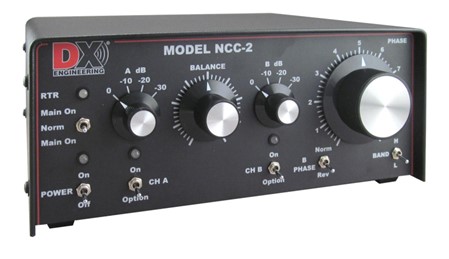
This was built around the DX Engineering NCC-2 Receive Antenna phasing unit and a matching pair of DX Engineering Receive Short Element Active Vertical Antennas (DXE-RSEAV-1).

My main interest is Weak Signal CW (Continuous Wave), which is the use of Morse code transmissions in conditions where signal strength is extremely low, often below the noise floor. My focus was on improving my Signal to Noise Ratio (SNR) particularly for 40 metres, which is my noisiest band. I also wanted to objectively measure the performance of the new system compared to my existing antenna.

To conduct this evaluation, I used a software suite called WSJT-X, developed by Joe Taylor, K1JT.

WSJT-X is widely used for weak-signal digital communication. It includes several modes designed for making reliable contacts under extreme conditions such as FT8, JT65 and WSPR. Each mode serves a
different purpose, but all are optimized for low power, low bandwidth transmissions that can be decoded even when signals are below the noise floor.

WSPR provides the ability to measure and evaluate receive (or transmit) performance. WSPR beacon stations around the world transmit 24 hours a day on most bands.

These stations can be received and the spots saved into an easily accessible global database. Combined with sophisticated but easy to use web tools, this provides the user with the ability to perform comprehensive analysis of station changes of any kind including new antennas, equipment, cabling or ground changes, or even antenna orientation.

This data is always available for retrieval at any later date and in the longer term provides the user with the ability to retrieve and compare changes to your station at any given time.

WSPR takes the guesswork out of antenna evaluation and with the new web tools to analyze and visualize results, measuring antenna performance is surprisingly very easy to do.

Test Setup for Antenna Comparison

Living on a small city lot, I have only had a single antenna for almost a decade. It is a carefully tuned Hustler 6BTV 6-Band HF Vertical Antenna with 68 radials, a high-quality DX Engineering current balun and good grounding. Combined with excellent low-loss UHF hardline, it has worked very well for me over the years.

Short of a tower and beam, I am satisfied that it is the best I can do in the limited space I have available.

To complement this, I installed a pair of DX Engineering RSEAV active receive-only vertical antennas along with an NCC-2 phasing unit which provides phasing and noise cancelling using two antennas.

The NCC-2 output was then connected to the RX antenna port of my TS-890. Next, I methodically started comparing relative receive performance between them and the 6BTV using WSPR to obtain
receive results of each.

When comparing two antennas, the most accuracy will result when signals are received from both antennas concurrently. This eliminates any short-term propagation changes skewing results. To do this, I configured my PC to run two instances of WSJT-X in WSPR mode as shown in Figure 1 and
Figure 2.

In one instance I connected it to my Kenwood TS-890 Transceiver and the new active verticals. In the other I connected it to an RSPdx-R2 SDR and the 6BTV.

Note: The SDRplay RSPdx-R2 is a single-tuner wideband full featured 14-bit SDR which covers the entire RF spectrum from 1 kHz to 2 GHz giving up to 10 MHz of spectrum visibility.

I then ran both instances of WSJT-X concurrently and collected WSPR data for extended periods, using the option to post my results to the WSPR database. Next, I used various web tools to do the heavy lifting to retrieve and analyze the wealth of information received.

I was able to investigate not only the number of stations received over a given period for each antenna, but also see the SNR of each, where they are located, direction, distance and so much more.

Gathering Data

Configuring two instances of WSJT-X each connected to its own antenna is done by creating two shortcuts to the application each with different targets (rig-name). For reporting purposes to the global WSPR database, it is necessary to add your call to one instance of WSJT-X and an alias to your call in the other instance.

For example, in my case, results were reported to the WSPR database as VE6JF on the receive verticals connected to my TS-890 (see Figure 1, above) and VE6JF/6 connected to my RSPdx-R2 SDR on the 6BTV (see Figure 2, above). I entered this on the “Settings”, “Reporting” tab in WSJT-X.

This naming convention lets me identify which data set belongs to which antenna. Don’t forget to enable reporting by checking the option “Upload Spots” on the main page in each instance. Following this, the WSPR spots you receive will then be uploaded to the WSPR database.

Note: For more detailed information on this method click here: Two Instances of WSJT-X Running Simultaneously with Two Radios Two Antennas

Data Analysis & Results

I used this WSPR comparison tool to query the WSPR database to view and analyze the data. This web application retrieves all columns in the database for the calls, band and time you select and then graphically shows how one antenna compares to the other.

While my main objective was SNR improvement, I decided to use “Spot Quality” (known as “SpotQ”) as my metric instead. This is a calculated number (always positive) that includes the SNR value of the spot received and directly represents how well a signal stands out from the noise.

While strictly not SNR alone, the SNR value received is included in the calculation and for my purposes it is a more granular and much better metric giving me a more complete measure of my overall system performance.

SpotQ represents the quality of any given spot using different transmit powers, distances and a normalized value of SNR. The formula is as follows:

SpotQ = (Distance(km)/Power(W)) * (SNR(dB)+35/35)

Distance/Power is straightforward. The value of 35 is used in the WSJT-X source code to set the minimum threshold for WSPR SNR Type 2 spots. By adding 35 and then dividing by 35 it ensures that the result will always be a number greater than 0.

The result, SpotQ, is a single, quantitative metric that allows for easier comparison of “how good” different WSPR spots are. If both my antennas hear the same transmitting station at the same exact time having identical k/W (kilometres per watt) and power levels, then the antenna with the lowest SNR (ie, highest SpotQ) that hears the station is the winner.

Figure 3 shows a graph of a 40 meter test and a comparison of SpotQ values reported for the 6BTV vs the new active verticals. The red trace represents the RSEAV verticals and the blue, the 6BTV.

The active verticals show a slight edge over the 6BTV and SpotQ results compare closely under quiet conditions. Later, testing performance under heavy QRN conditions will be described.

Digging a bit deeper beyond simple SNR measurements, I then examined my 40 meter results with another web tool, the Grafana Dashboard. This provides a 360-degree graphical view of reception (and more) for each antenna.

This is a different type of data view than in Figure 3 and can help a user decide on the best orientation and location for both receiving and transmit antennas.

In the example for 40 meters shown in Figure 4, I can see slightly improved coverage in the South (S) and Southeast (SE) direction with the active verticals (red) over the 6BTV (orange).

There are also many other ways to view data with wspr.rocks including charts and heat maps.

For the power user, there is also the ability to add custom SQL commands to further refine results based on parameters you choose. Customizing and building your own data queries is easily done and many examples are provided to get you started. It is also easy to copy and load WSPR results into Excel for further analysis, but I find wspr.rocks and Grafana sufficient for my purposes.

Note too, that propagation plays a large role as to which antenna performs better than the other at different times of day.

Occasionally, the 6BTV will hear more WSPR spots or even a higher SpotQ value than the active verticals. But due to the active verticals overall lower SNR, it is my antenna of choice as it greatly reduces operator fatigue for long CW sessions.

Noise would perhaps not be an issue for the FT8 operator, though a few dB of SNR improvement is always helpful with marginal signals.

Currently, with the active verticals installed I now only use the 6BTV for transmit.

The Return of QRN

All the above testing was done under quiet conditions, but that never lasts for long here. The improved receive capability of the active verticals becomes dramatically apparent under noisy conditions and I didn’t have to wait long for noise to return.

First, I adjusted the NCC-2 to null out my local QRN. Figure 5 shows the level of QRN I normally experience and Figure 6 shows the results after adjusting the NCC-2 phasing.

After nulling out the QRN, a test on 20 meters for several hours shows a spot count of 1523 for the active verticals (red) vs 715 for the 6BTV (blue). More importantly, the Spot Quality exceeds the 6BTV by a significant margin.

Note: Remember that SpotQ includes SNR in the calculation.

The graph shown in Figure 7 below indicates an improvement of 4 dB to 9
dB and sometimes more over an 8-hour period.

Contrasting these results with those under low noise conditions shown in Figure 3 that tracked more closely, demonstrates the active vertical advantage over the 6BTV under high noise conditions.

The number of additional spots heard are apparent.

A quick look at FT8 exchanges during this high QRN period reveals that in the CQ example in Figure 8, the station on the left with the active verticals was –2dB and the same one with the 6BTV was –22dB; a difference of 20dB.

Since the same SNR improvements are also observed with FT8, many more stations would have been workable.

In the presence of this QRN, the Grafana analysis pattern in Figure 9 shows the advantage of the active verticals (red) in their improved coverage.

Weaker stations further out were still being heard that were not discernible with the 6BTV (orange).

This and the above head-to-head testing in Figure 3 and Figure 7 dramatically demonstrates the power of WSPR for antenna comparison and detailed analysis, as well as the suitability of active verticals for lower SNR. Using WSPR gave me confidence that the changes to my new receive antenna system has made a measurable improvement.

Conclusion

In summary, using WSPR to measure signal strength and directionality between two antennas at the same time enabled me to objectively measure and compare my new receive antenna system against my existing 6BTV vertical.

While I have not done so, WSPR can be used in a similar fashion to test transmitting antenna effectiveness as well.

And of course, WSPR really excels when it comes to propagation analysis.

***

Jim Leslie, VE6JF was licensed in 1964 and built his first 80m rig from scavenged TV parts. Early on, he learned the hard way what high voltage can do to a person! After trying almost every mode there is, he always came back to CW, which has always been his favorite mode. He enjoys CW contests and was one of the CW ops in the 2025 RAC Canada Day Contest at the VE6SV Super Station operating as VE6RAC, as well as taking part in the CQWWDX CW contest there in past years. He enjoys operating POTA and is a member of the POTA support team. Mostly a homebrewer with a soft spot for test equipment, he has a fondness for building anything that involves RF and carefully measuring the results.

The post Measuring Antenna Performance Using WSPR appeared first on OnAllBands.